Advanced PID Controller Implementation
This content was kindly contributed by Dew Toochinda, the Scilab Ninja, and originally posted on https://scilabdotninja.wordpress.com/
In this digital era, PID controllers have evolved from basic textbook structure to more sophisticated algorithms. Features such as setpoint/derivative weightings and anti-windup scheme are often added to improve the closed-loop response. In our previous article A Decorated PID Controller, we consider a PID structure with modification and additional functions as follows
- To lessen the effect of measurement noise, derivative part is implemented as a filter with parameter N
- Back calculation anti-windup scheme is implemented with tracking gain Kt
- Setpoint weightings for proportional and derivative paths can be adjusted via Wp and Wd, respectively
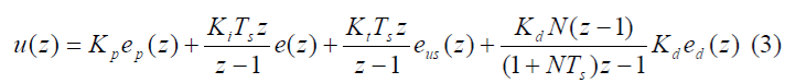
A feedback diagram with this advanced PID controller is constructed using Xcos palettes as in Figure 1. In equation form, this controller can be described as
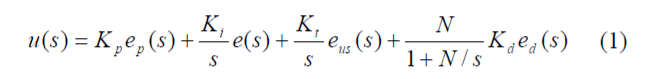
with
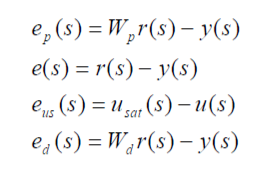
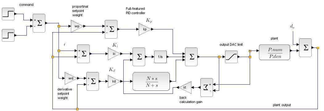
Figure 1 advanced PID feedback diagram
where r(s), y(s), u(s) and u_sat(s), are reference command, plant output, controller output, and saturated controller output, respectively. As described in our Discrete-time PID implementation article, using backward difference relationship
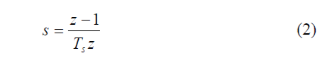
Equation (1) can be converted to z-domain as
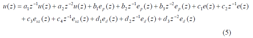
Rewrite (3) in terms of z-1

To implement this PID scheme as a computer algorithm, we have to convert (4) to a difference equation. It is straightforward to show that (4) can be rewritten as
with coefficients
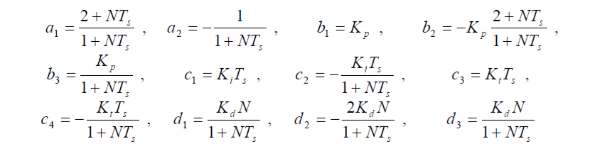
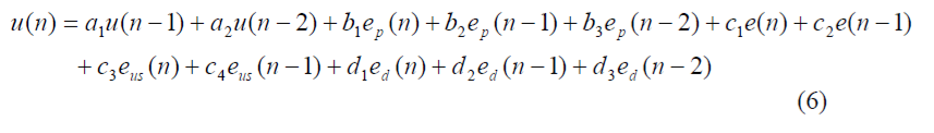
So the corresponding difference equation is
Response Comparison via Simulation
Equation (6) is ready for implementation on a target processor. Before that phase, we want to make sure that our equation and coefficients are without error. One easy way is to perform simulation on Xcos and compare the response to the original continuous-time PID controller. For this purpose, we construct a model advpid_imp.zcos as shown in Figure 2, consisting of 2 feedback loops. The upper loop is controlled by discrete-time PID in the form (5), and the lower loop contains the continuous-time PID. The simulation results from the two closed-loop systems are then compared to verify how well they match.
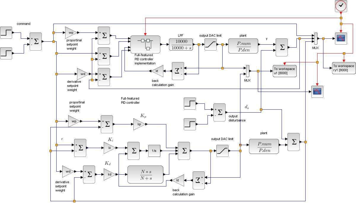
Figure 2 model advpid_imp.zcos for discrete and continuous PID comparison
Note that the discrete-time PID in the upper loop is contained in a superblock. The internal details are shown in Figure 3, which corresponds to the discrete-time controller (5).
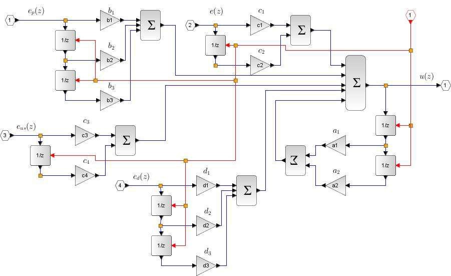
Figure 3 the internal details of discrete-time PID superblock
Also, at the output of discrete-time PID controller, a LPF transfer function is inserted to prevent an algebraic loop error, normally occurred with hybrid simulation. The LPF pole is chosen well above the closed-loop bandwidth so the filter does not have noticeable effect on the responses.
For easy editing, all the parameters in advpid_imp.zcos are initialized using a script file advpid_imp.sce. The plant is chosen as a third-order lag transfer function
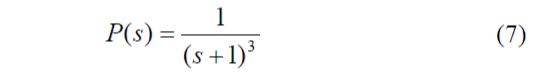
which can be created in Scilab by
s = poly(0,'s');

P = syslin('c',1/(s+1)^3);
Then, controller parameters are assigned values. These can be chosen as you like since the purpose of this simulation is to compare the responses. Here the PID gains are obtained from Zieglers Nichols frequency domain tuning method, and others are assigned some practical values.
kp = 4.8; |
// PID gains |
ki = 2.7; |
|
kd = 2.1; |
|
N = 10; |
// filter coefficient |
kt = 1.2; |
// back calculation gain for anti-windup |
wp = 0.7; |
// setpoint weight for proportional term |
wd = 0.1; |
// setpoint weight for derivative term |
Ts = 0.01; |
// sampling peroid |
For sampling period Ts, the value should match the simulation sampling period in the clock.
The parameters left to be assigned are the limits in saturation block. Put in some reasonable values such that some saturation effect happens during transient, since we prefer response comparison with the back calculation term activated. Too small the limit range would cause severe performance degradation. By some trial and error, we are finally satisfied with these values for saturation block
ulim = 2000;

llim = -2000;
Finally, the coefficients in (5) need to be computed. We introduce additional variables x1 and x2 for terms that appear in several places.
x1        = (1+N*Ts);

x2        = (2+N*Ts);

a1        = x2/x1;

a2        = -1/x1;

b1        = kp;

b2        = -kp*x2/x1;

b3        = kp/x1;

c1        = ki*Ts;

c2        = -ki*Ts/x1;

c3        = kt*Ts;

c4        = -kt*Ts/x1;

d1        = kd*N/x1;

d2        = -2*kd*N/x1;

d3        = kd*N/x1;
After all parameters are assigned, interactively or by executing advpid_imp.sce, we proceed by clicking on the simulation start button. The simulation results in Figure 4 show that the plant and controller outputs from continuous and discrete PID are almost identical. This makes us confident that the discrete-time PID and its coefficients are derived correctly.
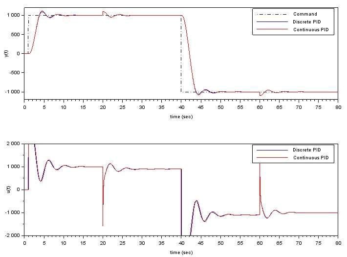
Figure 4 response comparison between continuous and discrete PID