Discrete-time PID Controller Implementation
This content was kindly contributed by Dew Toochinda, the Scilab Ninja, and originally posted on https://scilabdotninja.wordpress.com/
Download the files for this tutorial:
Part I: Discrete PID Gains as Functions of Sampling Time
In our previous article Digital PID Controllers, we discussed some basics of PID controller implementation as software algorithm on a computer. In that article, we simplify the matter by omitting the effect of sampling period on the PID parameters. In practice, we may want to relate a chosen set of parameters in continuous-time, perhaps from simulation or some tuning rule, to its discrete-time representation. In this article we investigate such relationship on a commonly-used PID form.
For the continuous-time PID, we start with the so-called parallel form
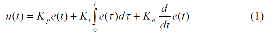
with its Laplace transform
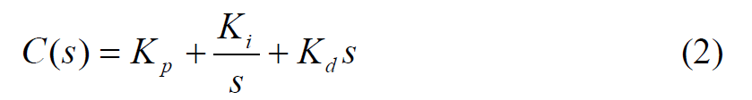
It is quite common to modify the derivative term to an LPF filter, to make it less noisy
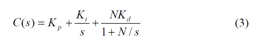
A straightforward way to discretize this controller is to convert the integral and derivative terms to their discrete-time counterpart. There are commonly 3 variations to do so, by means of forward Euler, backward Euler, and trapezoidal methods. Below we give representation for each.
Given a sampling period Ts ,the integral term Ki/s can be represented in discrete-from by
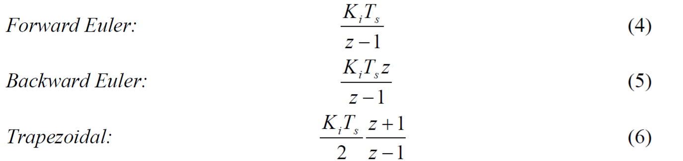
Similarly, the derivative term in (3) can be discretized as
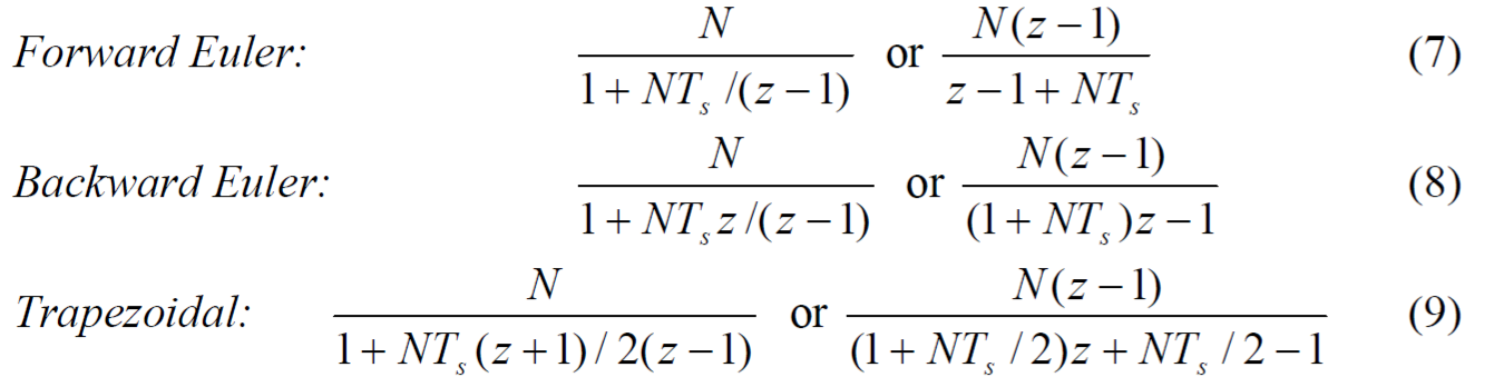
Obviously for all the terms above, the sampling period affects the gains of integral and derivative terms.
As an example, suppose we use backward Euler methods for both the integral and derivative terms, the resulting discrete-time PID controller is represented by
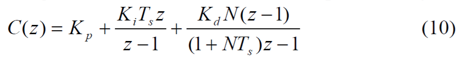
We want to simulate how this controller performs compared to its continuous-time version. We will use the setup in Figure 10 from our Module 4: PID Control. The plant consists of a robot joint driven by DC motor and a LPF at its input. Add the second feedback loop with discrete-time PID controller as shown in the Xcos diagram in Figure 1, or download dpidsim.zcos. Note that the controller is assembled from Xcos gain blocks, and the DLR blocks from discrete-time systems palette.
Kp = 200;           // these are values obtained from ZNFD tuning

Ki = 400;

Kd = 42;

Ts = 0.01; // must match sampling period used in simulation N = 20;
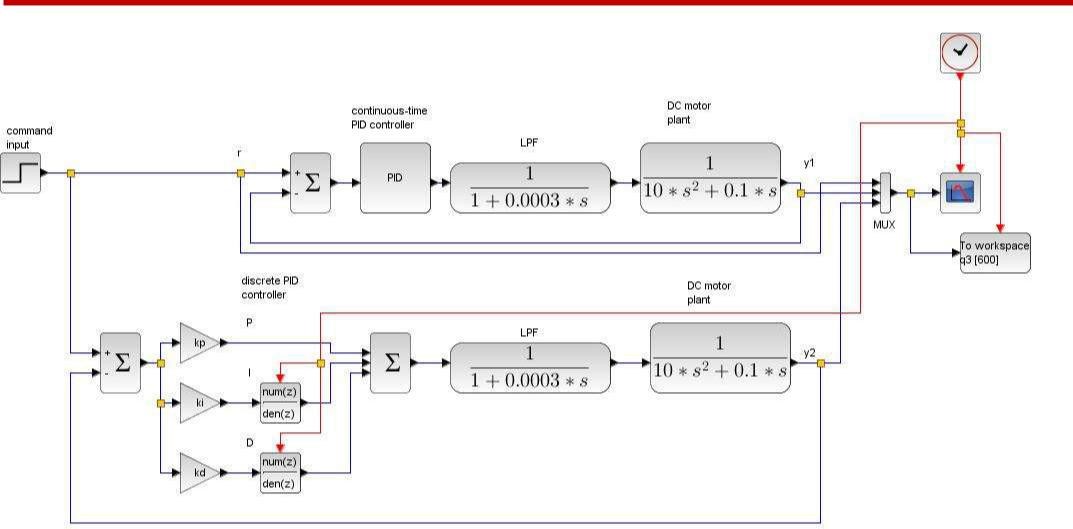
Figure 1 dpidsim.zcos continuous versus discrete PID simulation
Then the second and third terms from the controller expression in (10) is inputted to the DLR blocks for integral and derivative as shown in Figure 2 and 3, respectively.
Figure 2 integral block setup
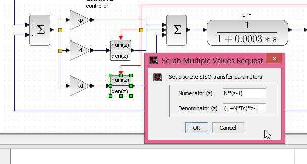
Figure 3 derivative block setup
Running the simulation yields the result in Figure 4. Notice that the step responses from the continuous (green) and discrete (red) PID controllers do not match, though they bear quite similar behavior.
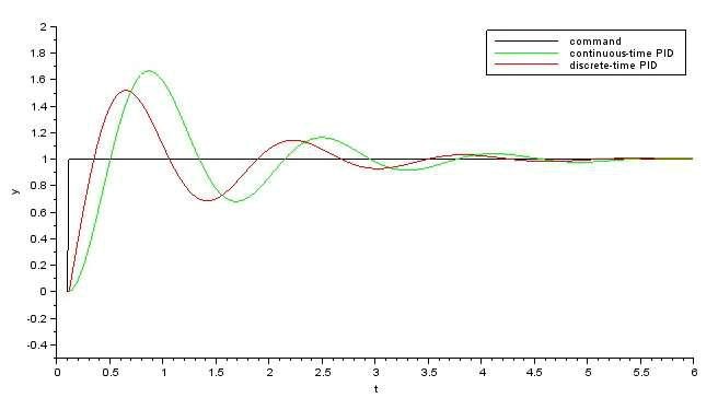
Figure 4 response comparison between the continuous and discrete PID
Of course, one would not expect a good match since the standard continuous-time PID block provided by Xcos does not have a filter in the derivative term. So to make a fair comparison, it takes some more work to construct a custom continuous-time PID controller according to (3) as shown in Figure 5.
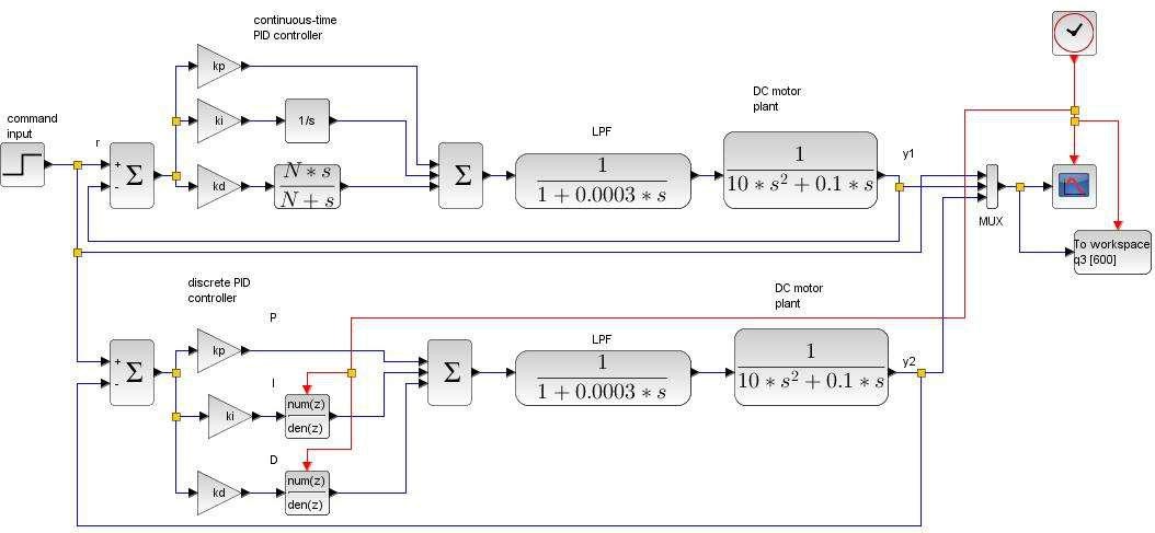
Figure 5 dpidsim2.zcos comparison with filter in the continuous-time PID controller
Download dpidsim2.zcos and run the simulation. The responses in Figure 6 depicts almost exact match between continuous and discrete PID control.
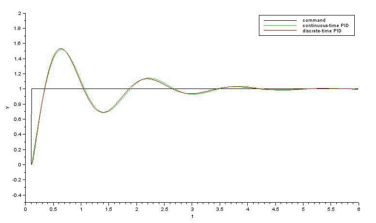
Figure 6 response comparison from dpidsim2.zcos
Conversion to PID Algorithm
In order to implement on a computer, a discrete-time controller in the Z-domain must be transformed to its difference equation from as explained in our previous article Digital PID Controllers. Only now the process becomes more involved because the sampling time is embedded in the gains. Also, our controller now has the filter in its derivative term. It is straightforward for the reader to verify that the discrete-time PID controller (10) can be manipulated into the form
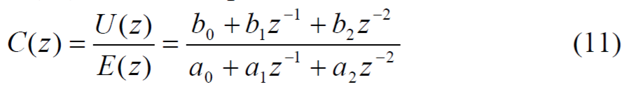
where U(z) and E(z) are controller output and input, respectively, and the coefficients are described by
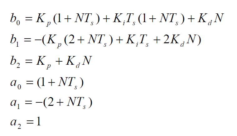
From (11), we rearrange
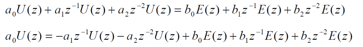
to yield the difference equation for controller output

To make sure that our coefficient computation is correct, we construct another Xcos model dpidsim3.zcos as shown in Figure 7, where the discrete-time PID is formed using (12). It is convenient to do the computation in a script file dpidsim3_setup.sce and execute it before simulation.
The response comparison in Figure 8 shows quite a good match between the algorithmic PID and its continuous-time representation, though the discrepancy is somewhat more noticeable than in Figure 6.
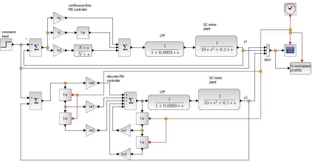
Figure 7 dpidsim3.zcos verification model for PID in algorithmic form
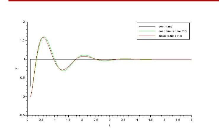
Figure 8 response comparison from dpidsim3.zcos
Equation (12) can be programmed easily using your choice of computer language. For example, in C it would appear as follow
// global variables

double e2, e1, e0, u2, u1, u0;                    // variables used in PID computation

double r;         // command

double y;        // plant output

//                    -- these parameters should be user-adjustable double Kp = 10; // proportional gain

double            Ki = 1;    //          integral gain

double            Kd = 1;   //          derivative          gain

N = 20;             //          filter coefficients

Ts = 0.01;       // This     must match      actual sampling time PID

//                    controller is running

//                    -- the following coefficients must be recomputed if

//                    --- any parameter above is changed by user

a0 = (1+N*Ts);

a1 = -(2 + N*Ts);
a2 = 1;

b0 = Kp*(1+N*Ts) + Ki*Ts*(1+N*Ts) + Kd*N;

b1 = -(Kp*(2+N*Ts) + Ki*Ts + 2*Kd*N);

b2 = Kp + Kd*N;

ku1 = a1/a0; ku2 = a2/a0; ke0 = b0/a0; ke1 = b1/a0; ke2 = b2/a0;

void pid(void) // implement this as timer interrupt service routine {

e2=e1; e1=e0; u2=u1;       u1=u0; // update variables

y = read();           // read    plant output

e0          = r –       y;           // compute new error

u0          = -ku1*u1            – ku2*u2 + ke0*e0 + ke1*e1 + ke2*e2; // eq (12)

if (u0     >            UMAX) u0          = UMAX;  // limit to DAC or PWM range

if (U0     <            UMIN) u0           = UMIN;

write(u0);            // sent    to output

}
Summary
In this article we discuss a practical discrete-time PID implementation, where the PID parameters are also functions of sampling time. The derivative term is commonly changed to an LPF to make it less noisy. Three conversion methods from continuous-time to discrete-time are generally used: forward Euler, backward Euler, and trapezoidal. Here we experiment only the backward Euler method. The reader is encouraged to simulate other methods and see which one gives the best match to continuous-time PID control.
We show in the last part how to implement a discrete-time PID controller as an algorithm on a computer or embedded system. In fact, the process can be applied to any type of controller described as a discrete-time transfer function in Z domain.
Exercises
- Show that a continuous-time PID controller in parallel form (2); i.e., without a filter in derivative term, can be discretized using trapezoidal (also called bilinear transform or Tustin) method as
Hint: Substitute 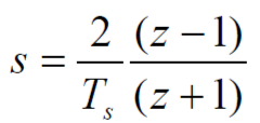 in (2) and collect terms
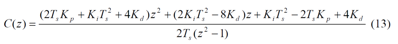
2. Implement the controller (13) using your choice of computer language.
Supplement
- dpid.zip : all Scilab and Xcos files used in this article
Revised History
March 2015: Correct the controller coefficient derivation and add dpidsim3.zcos to verify the result by response comparivon. Thanks to Manuel Brüderlin from Chair for Computational Analysis of Technical Systems (CATS) Aachen, who noticed that Kd was missing from the coefficient equations of (11).