Machine learning – Neural network classification tutorial

 

This tutorial is based on the Neural Network Module, available on ATOMS.
This Neural Network Module is based on the book “Neural Network Design” book by Martin T. Hagan.

Special thanks to Tan Chin Luh, for this outstanding tutorial, and the development of the Neural Network Module.

We will use the same data from the previous example: Machine learning – Logistic regression tutorial

 

Import your data

According to the previous tutorial mentioned earlier, yhis dataset represents 100 samples classified in two classes as 0 or 1 (stored in the third column), according to two parameters (stored in the first and second column):

data_classification.csv

 

Directly import your data in Scilab with the following command:

t=csvRead("data_classification.csv");

 

Represent your data

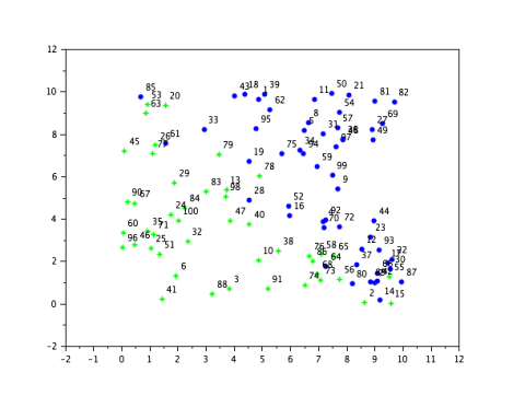
A function is implemented in neural network module to simplify the plotting of 2 groups of data points. First, we split the data to the source (P), and target (T). We transpose the data to match the format required by the module.

 P = t(:,1:2)';T = t(:,3)';plot_2group(P,T);

 

ANN Feed-Forward Backpropagation with Gradient Decent training function

Let’s try the FFBP with GD training algorithm. The full syntax is given as:

W = ann_FFBP_gd(P,T,N,af,lr,itermax,mse_min,gd_min)

 

where P is the training input, T is the training target, N is the number of neurons in each layer, including Input and output layer, af is the activation function from 1st hidden layer to the output layer, lr is the learning rate, itermax is the maximum epoch for training, mse_min is the minimum Error (Performance Goal) and gd_min is the minimum gradient for the training to stop.

 

On the left hand side, W representing the output weight and bias.

 

For simple, illustration, we just use the first 3 compulsory inputs, and others we left it empty to use the default values.

clear W;

tic();

W = ann_FFBP_gd(P,T,[2 3 1]);

toc()

y = ann_FFBP_run(P,W);

sum(T == round(y))

 

Scilab Console Output:

 

-->clear W;

-->tic();

-->W = ann_FFBP_gd(P,T,[2 3 1]);

-->toc()

ans =

   31.655

-->y = ann_FFBP_run(P,W);

-->sum(T == round(y))

ans =

74.

 

ANN Feed-Forward Backpropagation Gradient Decent with Adaptive Learning Rate and Momentum training function

In order to improve the convergence of the GD training, few methods were introduced in the book “Neural Network Design”. In this example, we will be using the combination of the adaptive learning rate and momentum training function.

 

The code is as follows:

clear W;
tic();
W = ann_FFBP_gdx(P,T,[2 3 1]);
toc()
y = ann_FFBP_run(P,W);
sum(T == round(y))

The training converges faster as compare to the previous GD example.

 

Scilab Console Output:

 

-->clear W;

-->tic();

-->W = ann_FFBP_gdx(P,T,[2 3 1]);

-->toc()

ans =

   38.829

-->y = ann_FFBP_run(P,W);

-->sum(T == round(y))

ans =

89.

ANN Feed-Forward Backpropagation Levenberg–Marquardt Algorithm Training Function

An even faster algorithm for convergence is the Levenberg-Marquardt Algorithm.

The code is as follows:

clear W;
tic();
W = ann_FFBP_lm(P,T,[2 3 1]);
toc()
y = ann_FFBP_run(P,W);
sum(T == round(y))

The result shows that the training converges in a few tens of iterations.

 

Scilab Console Output:

 

-->clear W;

-->tic();

-->W = ann_FFBP_lm(P,T,[2 3 1]);

-->toc()

ans =

   4.565

-->y = ann_FFBP_run(P,W);

-->sum(T == round(y))

ans =

90.

Visualize the results

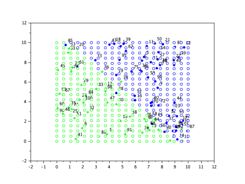
As the NN boundary could be complicated to be descripted in mathematics especially the neurons getting more in hidden layer (number of layers as well), visualising the boundary might be difficult.

So we will use the grid data which cover the range of the dataset to have the regions/boundary of the network

clf(0);
scf(0);
// Plot the data set
plot_2group(P,T);
// Create the input range grids
nx = 20; ny = 20;
xx = linspace(0,10,nx);
yy = linspace(0,10,ny);
[X,Y] = ndgrid(xx,yy);
// Use the trained NN to classify the grid data
P2 = [X(:)';Y(:)'];
y2 = ann_FFBP_run(P2,W);
// Extract the data according to the categories
G0 = P2(:,find(round(y2)==0))
G1 = P2(:,find(round(y2)==1))
// Plot the boundary and the region for the groups
plot(G0(1,:),G0(2,:),'go');plot(G1(1,:),G1(2,:),'bo');

 

What to Try Next?

The functions for the neural network module come with a brief description which could be access by the scilab help command. Trying different parameters could yield different results. More complicated datasets might needs different number of neurons/layers. Try it out!