Non Intrusive Spectral Projection Toolbox
Download the toolbox on:
http://atoms.scilab.org/toolboxes/NISP
Or the sources on:
https://gitlab.com/scilab/forge/nisp
Overview
An overview of the NISP toolbox.
Purpose
The goal of this toolbox is to provide Non Intrusive Spectral Projection method. It is related to the polynomial chaos tool in the OPUS platform, which received funding from the French National Research Agency (Agence Nationale de la Recherche). This toolbox is released under the LGPL licence.
Design
The internal design of the system is based on the following components :
-
“nisp” provides function to configure the global behaviour of the toolbox. This allows to startup and shutdown the library, configure and quiery the verbose level or initialize the seed of the random number generator.
-
“randvar” is the class which allows to manage a random variable. Various types of random variables are available, including uniform, normal, exponential, etc...
-
“setrandvar”, is the class which allows to manage a set of random variables. Several methods are available to build a sampling from a set of random variables. We can use, for example, a Monte-Carlo sampling or a Sobol low discrepancy sequence. This feature allows to use the class as Design of Experiment tool (DOE).
-
“polychaos” is the class which allows to manage a polynomial chaos expansion. The coefficients of the expansion are computed based on given numerical experiments which creates the association between the inputs and the outputs. Once computed, the expansion can be used as a regular function. The mean, standard deviation or quantile can also be directly retrieved.
The current toolbox provides an object-oriented approach of the C++ NISP library. This object oriented approach allows to manage objects, even if the Scilab language itself is not currently object-oriented (August 2009). This way, the Scilab toolbox accurately reflects the C++ library, without the need to manage memory (this is performed by the toolbox). To achieve this goal, the interface uses a hash map, which stores the map between integer tokens and the address of the associated C++ objects.
The current toolbox is a stand-alone component which uses only standard Scilab features.
Features
The following list presents the features provided by the NISP toolbox :
-
Manage various types of random variables :
-
uniform,
-
normal,
-
exponential,
-
log-normal,
-
-
Generate random numbers from a given random variable,
-
Transform an outcome from a given random variable into another,
-
Manage various sampling methods for sets of random variables,
-
Monte-Carlo,
-
Sobol,
-
Latin Hypercube Sampling,
-
various samplings based on Smolyak.
-
-
Manage polynomial chaos expansion and get specific outputs, including
-
mean,
-
variance,
-
quantile,
-
correlation, etc...
-
-
Generate the C source code which computes the output of the polynomial chaos expansion.
Example :
The following example is extracted from "Specifications scientifiques et informatiques : Chaos Polynomial", D-WP1/08/01/A, Martinez, CEA. In the following example, we compute the polynomial chaos expansion of a very simple function, taking two input variables and returning one output variable. The output result is computed by the Exemple function as the product of the two inputs. The first variable is associated with a Normal law, while the second is associated with a Uniform law.
The first step is to define the function to approximate.
function y=Exemple(x)
  // Returns the output y of the product x1 * x2.
  // Parameters
  // x: a np-by-nx matrix of doubles, where np is the number of experiments, and nx=2.
  // y: a np-by-1 matrix of doubles
  y(:,1) = x(:,1).* x(:,2)
endfunction
// 1. Two stochastic (normalized) variables
vx1 = randvar_new("Normale");
vx2 = randvar_new("Uniforme");
// 2. A collection of stoch. variables.
srvx = setrandvar_new();
setrandvar_addrandvar ( srvx,vx1);
setrandvar_addrandvar ( srvx,vx2);
// 3. Two uncertain parameters
vu1 = randvar_new("Normale",1.0,0.5);
vu2 = randvar_new("Uniforme",1.0,2.5);
// 4. A collection of uncertain parameters
srvu = setrandvar_new();
setrandvar_addrandvar ( srvu,vu1);
setrandvar_addrandvar ( srvu,vu2);
// 5. Create the Design Of Experiments
degre = 2;
setrandvar_buildsample(srvx,"Quadrature",degre);
setrandvar_buildsample( srvu , srvx );
// 6. Create the polynomial
ny = 1;
pc = polychaos_new ( srvx , ny );
np = setrandvar_getsize(srvx);
polychaos_setsizetarget(pc,np);
// 7. Perform the DOE
inputdata = setrandvar_getsample(srvu);
outputdata = Exemple(inputdata);
polychaos_settarget(pc,outputdata);
// 8. Compute the coefficients of the polynomial expansion
polychaos_setdegree(pc,degre);
polychaos_computeexp(pc,srvx,"Integration");
// 9. Get the sensitivity indices
average = polychaos_getmean(pc);
var = polychaos_getvariance(pc);
mprintf("Mean     = %f\n",average);
mprintf("Variance = %f\n",var);
S = polychaos_getindexfirst(pc);
mprintf("S1 = %f\n",S(1));
mprintf("S2 = %f\n",S(2));
ST = polychaos_getindextotal(pc);
mprintf("ST1 = %f\n",ST(1));
mprintf("ST2 = %f\n",ST(2));
// Clean-up
polychaos_destroy(pc);
randvar_destroy(vu1);
randvar_destroy(vu2);
randvar_destroy(vx1);
randvar_destroy(vx2);
setrandvar_destroy(srvu);
setrandvar_destroy(srvx);
There are many other demonstrations in the Demos: please open the Scilab Demonstrations and search for the NISP section.
The NISP User's Manual is provided in the doc directory in PDF format. In the following session, we get the path of the NISP module and display the list of documents available within the doc directory.
-->nisp_getpath()
 ans  =
 C:\Users\username\AppData\Roaming\Scilab\SCILAB~2.0\atoms\NISP\2.2-2
-->ls(fullfile(nisp_getpath(),"doc"))
 ans  =
!usermanual                                                !
!readme.txt                                                !
!OPUS_PC_Specifications_Fonctionnelles_V2-Martinez.doc     !
!nisp_toolbox_manual.pdf                                   !
!license.txt                                               !
!ChaosPolynomialSpecificationsFonctionnelles-Martinez.pdf  !
Authors
Copyright (C) 2012-2013 - Michael Baudin
Copyright (C) 2008-2011 - Jean-Marc Martinez - CEA
Copyright (C) 2008-2011 - INRIA - Michael Baudin
Copyright (C) 2004-2006 - John Burkardt
Copyright (C) 2000-2001 - Knut Petras
Copyright (C) 2002 - Chong Gu
Acknowledgments
Allan Cornet
Bibliography
"NISP Toolbox Manual", Michael Baudin (INRIA), Jean-Marc Martinez (CEA), Version 0.2, January 2011
"Polynomes de chaos sous Scilab via la librairie NISP", Michael Baudin (INRIA), Jean-Marc Martinez (CEA), 42emes Journees de Statistique, 24 au 28 mai 2010 - Marseille, France.
"The NISP module", https://scilab.gitlab.io/legacy_wiki/NISP_Module, Michael Baudin (INRIA), Jean-Marc Martinez (CEA), 2011
"Librairie NISP - Modelisation probabiliste d'incertitudes par developpement en chaos polynomial", JM. Martinez, CEA, RAPPORT DM2S, SFME/LGLS/RT/09-007/A.
GNU Lesser General Public License, http://www.gnu.org/copyleft/lesser.html
Distributions
In this section, we present the mean M and variance V of the random variables available in the randvar class. We also present the suppport of the random variables, i.e. the interval which contains the outcomes.
- "Normale"
-
The support is
(-%inf,+%inf).M=a V=b^2 - "Uniforme"
-
The support is
[a,b].M=(a+b)/2 V=(b-a)^2/12 - "Exponentielle"
-
The support is
[0,+%inf).M=1/a V=1/a^2 - "LogNormale"
-
The support is
[0,+%inf). The mean and standard deviation oflog(X)areaandb.If X is a LogNormale random variable with meanM=exp(a+b^2/2) V=(exp(b^2)-1)*exp(2*a+b^2)Mand varianceV, then:a=log(E)-0.5*log(1+V/E^2) b=sqrt(log(1+V/E^2)) - "LogUniforme"
-
The support is
[exp(a),exp(b)].If X is a LogUniforme random variable with minimumM=(exp(b)-exp(a))/(b-a) V=0.5*(exp(b)^2-exp(a)^2)/(b-a)-MAand maximumB, then:a=log(A) b=log(B)
Examples
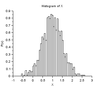
In the following example, we call the randvar_new function in order to create a Normal random variable with mean 1.0 and standard deviation 0.5. Then, we perform a loop so that we get 1000 values from this random variable. In order to check that these values are associated with a Normal distribution function, we compute the mean and variance and check that this corresponds to the expected results. Finally, the random variable is destroyed with the randvar_destroy function.
nisp_initseed(0);
mu = 1.0;
sigma = 0.5;
rv=randvar_new("Normale",mu,sigma);

nbshots = 1000;
values = zeros(nbshots);
for i=1:nbshots
values(i)=randvar_getvalue(rv);
end

mymean = mean (values);
mysigma = st_deviation(values);
myvariance = variance (values);

mprintf("Mean=%f (exact=%f)\n", mymean, mu);
mprintf("Std. dev.=%f (exact=%f)\n", mysigma, sigma);
mprintf("Var.=%f (exact=%f)\n", myvariance,sigma^2);

randvar_destroy(rv);

scf();
histplot(50,values)
xtitle("Histogram of X","X","P(x)")
The previous script produces the following output.

Example of randvar_getlog
In the following session, we use the randvar_getlog function and print a Normal variable in the console.
mu = 1.0;
sigma = 0.5;
rv=randvar_new("Normale",mu,sigma);
randvar_getlog(rv);
randvar_destroy(rv);
The previous script produces the following output.
      ***********************************************
      Nisp(RandomVariable::GetLog) for RandomVariable
      Normale : 1 : 0.5
      ***********************************************
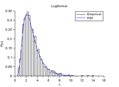
Example of Log-Normal variable.
In the following example, we create a Log-Normal variable. We compute the parameters from the parameters of the underlying Normal variable.
nisp_initseed(0);
a = 1.0;
b = 0.5;
rv=randvar_new("LogNormale",a,b);
nbshots = 1000;
values = zeros(nbshots);
for i=1:nbshots
values(i)=randvar_getvalue(rv);
end
// Check the mean of log(X)
mymean = mean(log(values))
expected = a
// Check the variance of log(X)
myvariance = variance(log(values))
expected = b^2
randvar_destroy(rv);
// Draw the histogram
scf();
histplot(50,values);
xtitle("LogNormal","X","P(x)");
// Compare with PDF
x = linspace(0,10,100);
p = distfun_lognpdf(x,a,b);
plot(x,p,"b-");
legend(["Empirical" "PDF"]);
The previous script produces the following output.

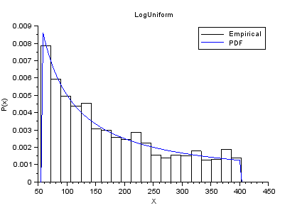
Example of Log-Uniform variable.
In the following example, we create a Log-Uniform variable. We compute the parameters from the parameters of the underlying Uniform variable.
nisp_initseed(0);
a = 4;
b = 6;
rv=randvar_new("LogUniforme",a,b);
nbshots = 1000;
values = zeros(nbshots);
for i=1:nbshots
values(i)=randvar_getvalue(rv);
end
// Check the mean of log(X)
mymean = mean(log(values))
expected = (a+b)/2
// Check the variance of log(X)
myvariance = variance(log(values))
expected = (b-a)^2/12
randvar_destroy(rv);
// Draw the histogram
scf();
histplot(20,values);
xtitle("LogUniform","X","P(x)");
x=linspace(exp(a),exp(b),100);
p=distfun_logupdf(x,a,b);
plot(x,p,"b-");
legend(["Empirical" "PDF"]);
The previous script produces the following output.

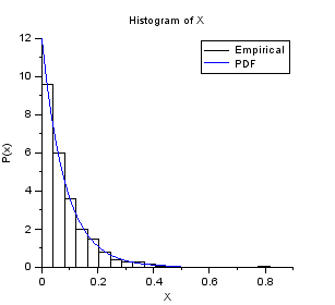
Example of Exponential variable.
nisp_initseed(0);
// Define a Exponential variable.
scale = 12.0;
rv=randvar_new("Exponentielle",scale);
// Perform Monte-Carlo simulations
nbshots = 1000;
values = zeros(nbshots);
for i=1:nbshots
values(i)=randvar_getvalue(rv);
end
// Check the mean
mymean = mean(values)
expected = 1/scale
// Check the variance
myvariance = variance(values)
expected = 1/scale^2
randvar_destroy(rv);
// Draw the histogram
scf();
histplot(20,values);
xtitle("Histogram of X","X","P(x)");
// Compare with PDF
x = linspace(0,0.5,100);
p = distfun_exppdf(x,1/scale);
plot(x,p,"b-");
legend(["Empirical" "PDF"]);
The previous script produces the following output.
Sampling Tutorial
A tutorial for the designs from setrandvar.
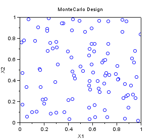
Monte-Carlo Sampling
In the following example, we create a "Monte-Carlo" sampling with 100 points in 2 dimensions, where each variable is uniform in [0,1].
srv=setrandvar_new(2);
setrandvar_buildsample(srv,"MonteCarlo",100);
sampling=setrandvar_getsample(srv);
scf();
plot(sampling(:,1),sampling(:,2),"bo");
xtitle("MonteCarlo Design","X1","X2");
setrandvar_destroy(srv)
The previous script produces the following output.

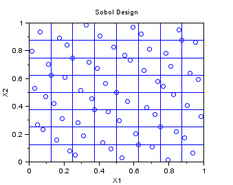
Quasi-Monte-Carlo Sobol Sampling
In the following example, we create a "QmcSobol" sampling with 63 points in 2 dimensions, where each variable is uniform in [0,1]. This is a Quasi-Monte-Carlo sequence, which can be used for multidimensionnal integration.
Notice that the first point, at (0,0) has been removed in the sample, so that there is no issue with the generation of samples from inversion of a cumulated distribution function. Indeed, if the point (0,0) has been kept, if normal variables were to be generated, for example, then the infinite point (-Inf,-Inf) would have been generated, which may cause a problem during the uncertainty propagation step, because the model would generate an infinite output.
We divide the unit square with squares with area 1/8 * 1/8=1/64. We can see that there is exactly one point in each cell. This is because the Sobol sequence is a (t,s)-sequence in base 2 with t=O(slogs). The Sobol sequence use the same base b=2 for all dimensions. This is why we can divide the space with elementary boxes based on a power of 2, so that the number of points in each box is constant. For more details on this topic, please use the "lowdisc" module for Scilab.
srv=setrandvar_new(2);
np = 63;
setrandvar_buildsample(srv,"QmcSobol",np);
sampling=setrandvar_getsample(srv);
scf();
plot(sampling(:,1),sampling(:,2),"bo");
xtitle("Sobol Design","X1","X2");
// Add the cuts
n=9
cut = linspace( 0 , 1,9);
for i = 1 : n
plot( [cut(i) cut(i)] , [0 1] , "-")
end
for i = 1 : n
plot( [0 1] , [cut(i) cut(i)] , "-")
end
setrandvar_destroy(srv)
The previous script produces the following output.

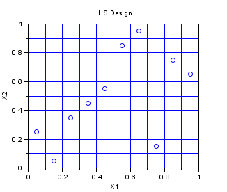
Latin Hypercube Sampling
In the following example, we create a Centered Lhs sampling for 10 points in dimension 2. The Lhs design which is provided in this module is a centered Lhs (which is different from the classical): as we can see, the points are in the center of each cell.
This is a design which is appropriate for multidimensionnal integration. The one-dimensional projections are as good as can be, in the sense that the design guaranties that at leat one point is in each cell. If the code is monotone with respect to its arguments, then the LHS design improves the accuracy of the estimate of the mean, by reducing the variance of the estimator.
srv=setrandvar_new(2);
np = 10;
setrandvar_buildsample(srv,"Lhs",np);
sampling=setrandvar_getsample(srv);
scf();
plot(sampling(:,1),sampling(:,2),"bo");
xtitle("LHS Design","X1","X2");
// Add the cuts
cut = linspace( 0 , 1,np + 1);
for i = 1 : np + 1
plot( [cut(i) cut(i)] , [0 1] , "-")
end
for i = 1 : np + 1
plot( [0 1] , [cut(i) cut(i)] , "-")
end
setrandvar_destroy(srv)
The previous script produces the following output.

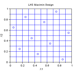
LHS Maximin
In the following example, we create a Centered Lhs-Maximin sampling for 10 points in dimension 2. We select the best sampling in a set of 1000 samplings, so that the minimum distance between two points in the sampling is maximized. The Lhs design which is provided in this module is a centered Lhs (which is different from the classical): as we can see, the points are in the center of each cell.
This is a design which is appropriate for multidimensionnal integration. It has all the good properties of a LHS design and has, potentially, a better space-filling property. Indeed, the figure below has points which are more regularily distributed in the 2D space than that previous LHS design.
srv=setrandvar_new(2);
np = 10;
setrandvar_buildsample(srv,"LhsMaxMin",np,1000);
sampling=setrandvar_getsample(srv);
scf();
plot(sampling(:,1),sampling(:,2),"bo");
xtitle("LHS Maximin Design","X1","X2");
// Add the cuts
cut = linspace( 0 , 1,np+1);
for i = 1 : np + 1
plot( [cut(i) cut(i)] , [0 1] , "-")
end
for i = 1 : np + 1
plot( [0 1] , [cut(i) cut(i)] , "-")
end
setrandvar_destroy(srv)
The previous script produces the following output.

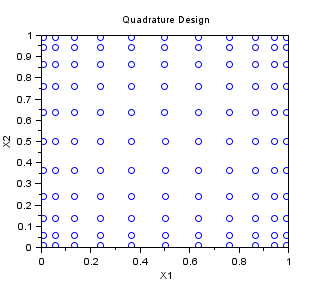
Quadrature
In the following example, we create a "Quadrature" sampling for np=10 in dimension 2. The one-dimensionnal Gauss quadrature rule has np+1 points. It is tensorised, so that the final 2D sampling has (np+1)^2 points.
srv=setrandvar_new(2);
np=10;
setrandvar_buildsample(srv,"Quadrature",np);
sampling=setrandvar_getsample(srv);
scf();
plot(sampling(:,1),sampling(:,2),"bo");
xtitle("Quadrature Design","X1","X2");
setrandvar_destroy(srv)
The previous script produces the following output.

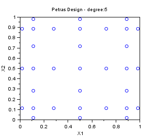
Petras
In the following example, we create a "Petras" sampling for maxdegree=5 in dimension 2. The Smolyak algorithm is so that the PC decomposition is exact for a polynomial with degree maxdegree. Notice that the number of points is greatly reduced with respect to a "Quadrature" sampling.
srv=setrandvar_new(2);
maxdegree=5;
setrandvar_buildsample(srv,"Petras",maxdegree);
sampling=setrandvar_getsample(srv);
scf();
plot(sampling(:,1),sampling(:,2),"bo");
xtitle("Petras Design - degree:5","X1","X2");
setrandvar_destroy(srv)
The previous script produces the following output.

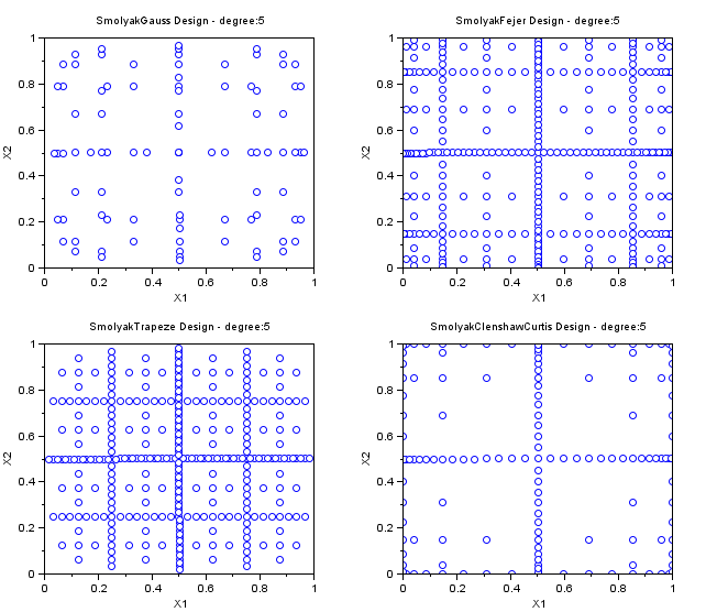
Other Smolyak Designs
In the followings example, we create various Smolyak samplings for maxdegree=5 in dimension 2. These SmolyakGauss algorithms are so that the PC decomposition is exact for a polynomial with degree maxdegree. Notice that the number of points is greatly reduced with respect to a "Quadrature" sampling.
- The "SmolyakGauss" sampling computes a multi-dimensional sparse grid based on a Gauss one-dimensional formula.
- The "SmolyakTrapeze" sampling computes a multi-dimensional sparse grid based on a Trapezoidal one-dimensional formula.
- The "SmolyakFejer" sampling computes a multi-dimensional sparse grid based on a Fejer one-dimensional formula.
- The "SmolyakClenshawCurtis" sampling computes a multi-dimensional sparse grid based on a Clenshaw-Curtis one-dimensional formula.
- This one-dimensional formula uses absissas based on the roots of Chebyshev polynomials.
names=[
"SmolyakGauss"
"SmolyakFejer"
"SmolyakFejer"
"SmolyakClenshawCurtis"
];
maxdegree=5;
scf();
for i=1:4
subplot(2,2,i);
srv=setrandvar_new(2);
setrandvar_buildsample(srv,names(i),maxdegree);
sampling=setrandvar_getsample(srv);
plot(sampling(:,1),sampling(:,2),"bo");
xtitle(names(i)+" Design - degree:"+string(maxdegree),..
"X1","X2");
setrandvar_destroy(srv);
end
The previous script produces the following output.

Number of experiments in quadrature samplings
In the followings example, we compute the number of experiments in various quadrature-type samplings.
names=[
"Quadrature"
"Petras"
"SmolyakGauss"
"SmolyakFejer"
"SmolyakTrapeze"
"SmolyakClenshawCurtis"
];
for maxdegree=1:9
mprintf("maxdegree=%d\n",maxdegree)
for i=1:6
srv=setrandvar_new(2);
setrandvar_buildsample(srv,names(i),maxdegree);
sampling=setrandvar_getsample(srv);
np=size(sampling,"r");
setrandvar_destroy(srv);
mprintf("    %s, np=%d\n",names(i),np)
end
end
| maxdegree | Quadrature | Petras | SmolyakGauss | SmolyakFejer | SmolyakTrapeze | SmolyakClenshawCurtis |
| 1 | 4 | 5 | 5 | 5 | 5 | 5 |
| 2 | 9 | 9 | 14 | 17 | 17 | 13 |
| 3 | 16 | 17 | 30 | 49 | 49 | 29 |
| 4 | 25 | 33 | 55 | 129 | 129 | 65 |
| 5 | 36 | 33 | 91 | 321 | 321 | 145 |
| 6 | 49 | 65 | 140 | 769 | 769 | 321 |
| 7 | 64 | 97 | 204 | 1793 | 1793 | 705 |
| 8 | 81 | 97 | 285 | 4097 | 4097 | 1537 |
| 9 | 100 | 161 | 385 | 9217 | 9217 | 3329 |
| 10 | 121 | 161 | 506 | 20481 | 20481 | 7169 |