Xcos Blocks Seasoning

This content was kindly contributed by Dew Toochinda, the Scilab Ninja, and originally posted on https://scilabdotninja.wordpress.com/

 

Download the files for this tutorial:

Time to continue our exploration. In this document we focus on Xcos and some useful blocks it provides. The Xcos diagram is pretty much the same as the one used in Recipe 2. Only the controller is changed to PID block for simplicity. So the diagram is renamed to mypidx.zcos, where x is an index number 1 or 2.

The plant data is also retained. Here we create it once again.

--> s=poly(0,'s')
 s  = 

    
   s

--> P = syslin('c',P)
 P  = 

              
      2       
   ---------  
           2  
   0.5s + s   

The first common task we want to explore is how to transfer data between Xcos diagram and Scilab workspace.

From/To Workspace Block

There are two primary blocks in the sources and sinks palettes of Xcos that we can use: FROMWSB (From workspace) and TOWS_c (To workspace). Let’s add them to the Xcos diagram as shown in Figure 1. Name this diagram mypid1.zcos.

To have the same results as shown in this article, perform the following parameter setups.

Click on Simulation -> Setup, adjust final integration time to 10 secs. Also change the refresh period in the scope to match

Double click on the red clock. Adjust Period to 0.01 and Initialisation time to 0.

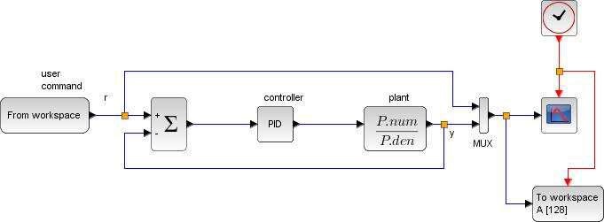
Figure 1 PID feedback diagram with From/To Workspace blocks [mypid1.zcos]

Do not run the simulation at this time because there is no command input. Double click on the From workspace block to see what data and parameters it needs. You would see the parameter window as in Figure 2 with 4 input fields. For this basic tutorial, we only need to specify a variable name. Put r in the variable name field. This tells Xcos to look for a variable name r in Scilab workspace, which we have to create later on.

Next, do the same with To Workspace block. Double click to launch the parameter window as shown in Figure 3. Type ry as the variable name and set buffer size to 1000. You may wonder where this number comes from. It’s just the total number of points generated from simulation. So 1000 points are the result of 10-second simulation with sampling period 0.01.

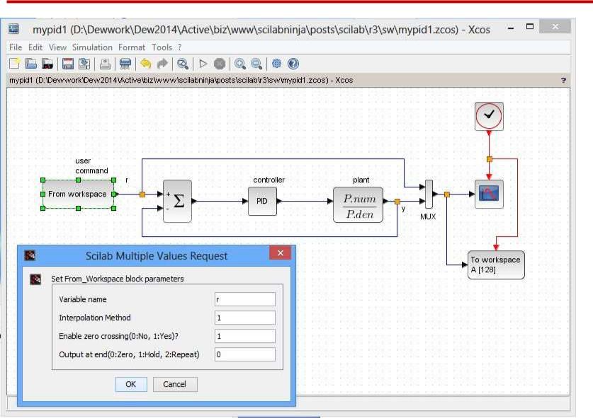
Figure 2 From Workspace block parameters window

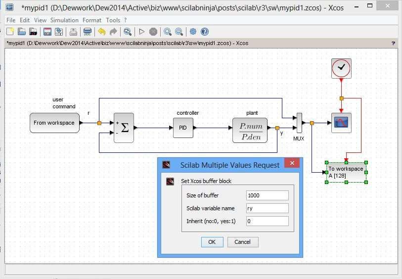
Figure 3 To Workspace block parameters window

From/To Workspace Data Format

A variable Xcos could read via From Workspace block must be a data structure with two fields: time and values. The data in these fields must be arranged column-wise; i.e., for n data points, the size of time field is n x 1 and size of values field is n x m (for m input channels; in our case m = 1). The output variable from To Workspace block is also generated in similar format. For mypid1.zcos diagram, the output values contain 2 channels: r and y. So r and y data are contained in ry.values(:,1) and ry.values(:,2), respectively.

For example, suppose we want to put a constant value 1 as input throughout the total 10-second time, the command input variable r can be generated as follows

--> r.time = (0.01:0.01:10)';

--> r.values = ones(1000,1);

Notice the transpose operation in r.time generation.

This input can be generated by a step function block. To make the From Workspace worthwhile, let us generate some command that cannot be achieved by a standard block. Suppose at t=0 we want a narrow, positive pulse command of magnitude 100 with duration 0.1 second. Then at t = 5 seconds, a negative pulse of magnitude -100 and same duration is applied.

For this customized input, the r.time data can still be generated as above. But now we need to do more work with the values of r. Here is a way to obtain

--> r.values=zeros(1000,1); // start with all zeros

--> r.values(1:10,1) = 100; // r = 100, 0 < t <=0.1

--> r.values(501:510,1) = -100; // r = -100, 5.0 < t <= 5.1

--> plot(ry.time,ry.values(:,1),'b-',ry.time,ry.values(:,2),'r-');

--> xlabel('time (sec)');

--> ylabel('y(t)');

--> legend('Command r(t)','Output y(t)');

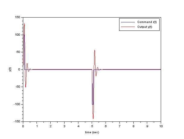
Figure 4 Command v.s response plot from data obtained in ry variable

Now we know how To/From Workspace blocks work. Let’s examine some others.

More blocks mean more fun.

Effects of Saturation

Saturation is a nonlinear element that normally exists in real applications, because most physical quantities have their limits. A digital controller implemented on modern microcontroller may have its A/D that accepts input voltage not exceeding 3.3 volts, say. This nonlinearity could have detrimental effects on a feedback system. Performance may be severely degraded or, for the worst case, the closed-loop system may even go unstable when limits are imposed somewhere in the loop. In this section we investigate these saturation effects.

Scilab provides a SATURATION block in Discontinuities palette. In mypid2.zcos shown in Figure 5, the block is placed at the PID controller output, together with a selector switch (SWITCH_f block from Signal Routing palette). So we can connect/disconnect the saturation with this switch, by double clicking on the switch block and choose the value in connected input filed between 1 or 2.

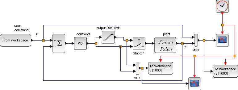
Figure 5 PID feedback diagram with controller output limit [mypid2.zcos]

The output limit is set to + 2047, a range for 12-bit DAC or PWM. Double click on the saturation block to input these upper and lower limits. The PID gains are reduced to P = 100, I = 10, D = 5, because high gains from last example destabilizes the closed-loop system when saturation is in effect.

To compare the responses, we have to run the simulation twice. For the first time, connect the selector to input 1 (saturation is active). Put a number index to the two output variables in To Workspace blocks as u1 and ry1. Run the simulation and wait until it ends. Now we have the first dataset u1 and ry1 corresponds to the feedback with saturation case.

Next, select input 2 at the switch, change the output variable names to u2 and ry2.

Run the simulation to get the second dataset.

Now perform the following plots for comparison.

--> subplot(211),plot(ry1.time,ry1.values(:,1),'b-',ry1.time,ry1.values(:,2),'r-',ry2.time,ry2.values(:,2),'g-');

--> xlabel('time (sec)');

--> ylabel('y(t)');

--> legend('Command','y(t) with saturation','y(t) w/o saturation',4);

--> subplot(212),plot(u1.time,u1.values(:,1),'r-',u2.time,u2.values(:,1),'g-');

--> xlabel('time (sec)');

--> ylabel('u(t)');

--> legend('u(t) with saturation','u(t) w/o saturation',4);

This yields the plots in Figure 6. We see clearly the response when saturation is present (red) degrades from the pure linear feedback case (green). The effects get even worse with the use of integral term in a PID controller such that it bears a term integrator windup. Some anti-windup scheme is normally implemented in a commercial PID controller to combat this undesirable response degradation.

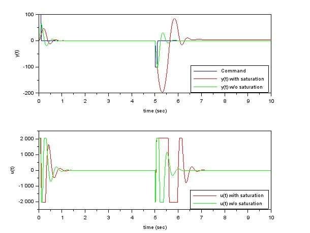
Figure 6 plots from mypid2.zcos that shows effects from saturation

There are so many blocks in the Xcos palettes, from basic to advanced, waiting for you to discover. Some I have not tried myself. Nevertheless, I hope you now get some idea on how to use them in a diagram, because the process is pretty much the same; i.e., drag one to your diagram, make connections, and setup its parameter(s). The red port goes with red, black with black, input to output, and vice versa. There are also those Modelica-based Electrical and Thermo-Hydraulics that have rectangular ports and require a C compiler to run. Those are beyond the discussion in this article.

Supplement

Scilab and Xcos files used

mypid1.zcos the Xcos diagram in Figure 1 mypid2.zcos the Xcos diagram in Figure 5

mypid.sce a Scilab setup script (for Xcos diagram initialization, in case you are lazy to type or copy/paste the commands embedded in the article.)