PID Anti-Windup Schemes
This content was kindly contributed by Dew Toochinda, the Scilab Ninja, and originally posted on https://scilabdotninja.wordpress.com/
Download the files for this tutorial:
Integrator windup in PID feedback control is well-known to control engineers. It happens when the integral term is used with some nonlinear saturation in the loop, such as when a physical variable reach its limit. When that happens, the feedback loop breaks, causing error accumulation in the integrator. This results in worse step and disturbance responses than the case of pure linear system.
To combat with the detrimental windup effects, a commercial PID controller often has some additional function called anti-windup. There are variations of implementation out there. Here we only investigate two basic schemes: conditional integration and back calculation.
Before further discussion, we have to review the two commonly-used forms of PID. First,
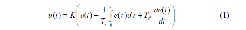
is often referred to as the textbook form. The second one is the parallel form used in Scilab Xcos block
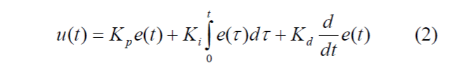
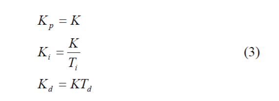
Some tuning methods such as Ziegler Nichols use the form (1). In this article we prefer (2). This variation should not pose a problem since the parameters between the two can be related by
The plant used is the same one from our Digital PID Controllers article.

which we already performed parameter tuning in that article. Those parameters will be used in the simulation.
Effects of Integrator Windup on Step Response
To see how integrator windup deteriorates the step response, we use an Xcos diagram mypid.zcos shown in Figure 1. An output limit block is connected to the PID controller output, which can be switched on/off by a selector. The saturation is set up to + 511, a limit for 10-bit DAC or PWM. Further discussion of this setup can be read from our Scilab Recipe 2: Xcos Block Seasoning.
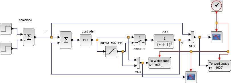
Figure 1: Xcos diagram with saturation block [mypid.zcos]
Setup the PID block by parameters achieved from the ZNFD tuning in Digital PID Controllers, and converted by (3).
ku = 8;        // ultimate gain

tu = 3.5;         // oscillation period

kp = 0.6*ku;          // PID controller gains

ki = kp/(0.5*tu);

kd = 0.125*kp*tu;
The command input is a switching step command that starts from 0 to 1000 units at t=0.1 sec and switch to – 1000 units at t=20 secs. Run the simulation twice, first time as pure linear system (switch connected to input 1) and second time with output limit in effect (switch connected to input 2). Save the data to different variable names and plot a comparison. The result is shown in Figure 2. Notice that the windup effect for this system does not cause higher overshoot, but degrades significantly the rise time of step response.
To implement anti-windup, we will have to add extra mechanisms into our PID controller. So instead of using the PID block from Scilab palette, we have to construct our own, which is not difficult to do. Furthermore, the modified structure from our article Discrete-time PID Controller Implementation is used; i.e., the derivative part is replaced by Low-pass Filter for better noise immunity.
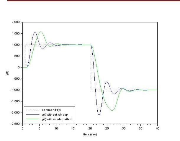
Figure 2 response comparison from mypid.zcos
Scheme1: Conditional Integration
The idea of conditional integration scheme is simple. Whenever there is some indication that saturation is causing error accumulation, the integrator in PID controller is turned off. There is however some variation in deciding when to switch off. The easiest one to implement is perhaps monitoring the controller output and comparing with the limits. Whenever saturation occurs, the integrator is turned off.
The Xcos model awupid_m1.zcos in Figure 3 is built to experiment with this conditional integration scheme, implemented in the lower feedback diagram. The plant now accepts data from a linear system P in Scilab workspace. So you can easily use the model with some other plant by constructing a new P. At this point we still use (4)
--> s = poly(0,'s');

--> P = syslin('c',1/(s+1)^3);
Notice that the derivative is implemented as an LPF with additional parameter N. We choose this as some large value, say
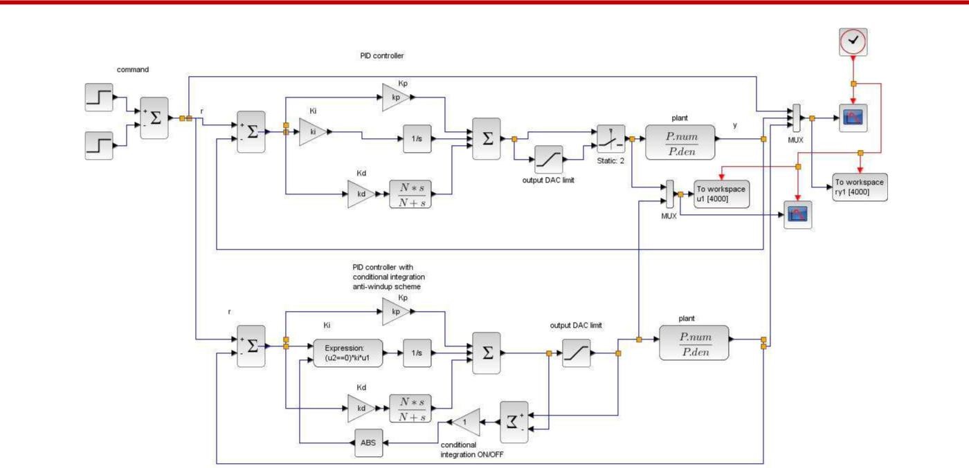
Figure 3 PID control with conditional integration scheme [awupid_m1.zos]
-->N = 1000;
Other PID gains remain the same as above.
Note: For your convenience, all setups are contained in a script file awupid.sce. Run the script once before simulation.
-->exec('awupid.sce',-1);
To see a comparison, connect the selector switch in the upper diagram to input 2. That routes the PID controller output through the output DAC limit block. Then click run. Figure 4 is the resulting scope view of output responses. Tracking performance is significantly improved with the conditional integration scheme, in
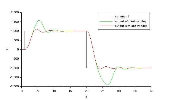
Figure 4 output responses from awupid_m1.zcos
the sense of overshoot reduction. However, it could not improve the rise-time of step response that degrades from the pure linear system.
There is no parameter to adjust in the conditional integration scheme. The integrator is simply switched on or off depending on whether a signal saturates.
Scheme 2: Back Calculation
Back calculation anti-windup scheme can be viewed as supplying a supplementary feedback path around the integrator. This feedback becomes active and helps stabilize the integrator only when the main feedback loop is open due to saturation. To experiment with this scheme, use an Xcos model awupid_m2.zcos in Figure 5. The back calculation feedback is implemented in the lower diagram, with additional compensation gain kt.
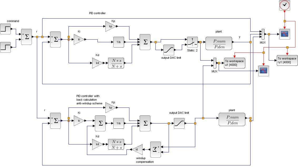
Figure 5 PID control with back calculation scheme [awupid_m2.zos]
Figure 6 shows five output responses with kt = 0.1, 0.5, 1, 2, 5. The overshoot lessens with increasing kt, though too large a value causes slower rise-time, and even induces undershoot for the case kt = 5.
Similar to the conditional integration scheme, rise-time cannot be improved to match the case of pure linear system.
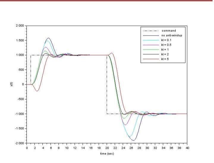
Figure 6 output responses from awupid_m2.zcos
Conclusion
In this article, we discuss two anti-windup schemes in a PID controller and simulate some closed-loop step responses with a chosen plant transfer function. The audience can download Xcos files and perform further investigation with other choices of parameters and plants. We would also be interested to learn how these schemes behave under more realistic situations, such as tracking performance with other command inputs, with added input/output disturbances, or operating under noisy condition, etc.
References
- K.J. Astrom and T.Hagglund. Advanced PID Control Instrumentation, Systems, and Automation Society, 2006.
- V. Toochinda. Digital PID Controller, 2011.
- V. Toochinda. Module 4: PID Control, in Scilab Control Engineering Basics, Scilab.Ninja, 2014.
Supplement
Scilab and Xcos files used:
mypid.zcos Xcos diagram in Figure 2
awupid_m1.zcos Xcos diagram in Figure 3
awupid_m2.zcos Xcos diagram in Figure 5
awupid.sce Scilab setup script